Simple application for solid state NMR to model polarization transfer kinetics (ver 1.0.17).
This tool combines the physics of solid-state NMR with robust statistical methods to help you extract meaningful, reliable kinetic parameters from your experimental data.
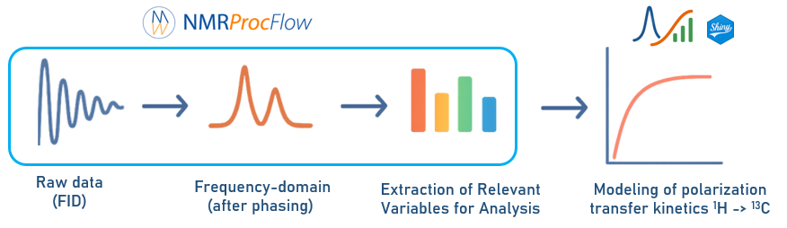
Enter a Tab-Separated Values (TSV) file corresponding to a bucket matrix resulting from processing by the NMRProcFlow application of solid-state NMR spectra (CP pulse sequence). See Tutorial on using NMRProcFlow to produce the polarization transfer kinetics matrix. See also an overview of the complete workflow.
Quick Help
Funded by
Main contributors
- Daniel Jacob, Xavier Falourd, Catherine Deborde
License
- GNU GENERAL PUBLIC LICENSE Version 3, 29 June 2007 - See http://www.gnu.org/licenses/ for more details.
Citation
- D. Jacob, X. Falourd, C. Deborde, M. Lahaye, C. Rondeau-Mouro (2026) “A Reproducible Workflow for Modelling of 1H to 13C Polarization Transfer Kinetics using Solid-State NMR”, Magnetic Resonance in Chemistry, doi:10.1002/mrc.70090
Purpose
This application allows you to model and analyze proton-to-carbon transfer kinetics from solid-state NMR experiments. It uses data extracted from NMRProcFlow [1] (a TSV - Tab-Separated Values - file corresponding to a bucket matrix ) resulting from processing by the ERVA (Extraction of Relevant Variables for Analysis) [2] approach to identify relevant buckets (corresponding to C₁–C₆).
See online documents :
- Tutorial on using NMRProcFlow to produce the polarization transfer kinetics matrix in Solid-State NMR.
- Overview of the complete workflow.
The app fits kinetic transfer curves (e.g. C₁–C₆ carbons) using nonlinear least-squares modeling modeling relying on Levenberg–Marquardt algorithm and provides a full suite of goodness-of-fit, predictivity, parsimony, sensitivity, and robustness analyses.
In short, it helps you to :
-
fit appropriate kinetic models to your experimental curves,
-
quantify the quality and reliability of each fit,
-
evaluate how robust and identifiable your fitted parameters are.
User Inputs (Interface)
The main controls in the Shiny interface allow you to tailor the modeling procedure:
| Parameter | Description / Purpose |
|---|---|
| Bucket/compound to model | Select the variable (i.e bucket or a compound) you want to analyze |
| Model | Choose the kinetic model to fit (the corresponding equations are given into the ‘Models’ tab) |
| Parameter constraints | Fixe the value range [min, max] for each parameter |
| Maximum contact time | Define the upper limit of the time range used for fitting (depending on the model and/or if the modeling is partial or total) |
| Number of fits | Specify how many model fits to perform (helps evaluate stability and reproducibility) |
| Residual threshold | Set a cutoff for excluding outlier points based on residuals before refitting (useful to reduce the influence of experimental noise) |
| Bootstap samples | Number of bootstrap resamplings to estimate parameter robustness and confidence intervals. |
So the steps to follow in order are: :
- Select the variable to analyze
- Choose a kinetic model (see Models tab).
- Choose the maximum contact time (depending on the model).
- Set parameters:
- Number of model estimations
- Residual threshold (exclude outliers)
- Number of bootstrap samples
- Run the model fit and interpret the outputs below.
Modeling Method
Model fitting is performed using the Levenberg–Marquardt algorithm (nlsLM function from the R minpack.lm package [3]). This algorithm minimizes the difference between the experimental data and the model prediction to estimate the kinetic parameters.
- This algorithm combines the strengths of the Gauss–Newton and gradient descent methods, making it robust for nonlinear kinetic models.
- You can apply constraints (i.e value range [min, max] for each parameter).
Each fit estimates model parameters by minimizing the Residual Sum of Squares (RSS) between the observed data and the model.
Outlier removal can be performed by applying a threshold to the residuals corresponding to the number of times their standard deviation (value between 2 and 3) after unfiltered modeling.
- This allows for the elimination of the few extreme values that could adversely affect the optimization.
- Caution: Some points may be considered extreme if the model is not suitable. Thus, information not taken into account by the model may be found in the residuals. Particular attention should be paid to the first points, especially if the polarization transfer is rapid.
- A value of zero indicates no filtering.
Results and Interpretation
The app provides several categories of results:
1. Fit Quality
| Metric | Meaning | How to interpret |
|---|---|---|
| RSS | Measures the overall deviation between model and data | Lower = better fit |
| R² (adjusted) | Fraction of variance explained by the model | Values near 1 indicate a good fit; adjusted R² corrects for overfitting |
| RMSE (Root Mean Square Error) | Average deviation between model and observations, same unit as data | Lower = more accurate fit. |
| MAE (Mean Abs. Error) | Mean absolute prediction error, less sensitive to outliers than RMSE | Lower = better predictive accuracy. |
| AIC / BIC | Information criteria balancing fit quality and model complexity. | Lower = better trade-off between accuracy and simplicity. |
➡️ Good fit: high R², low RMSE, low AIC/BIC.
Note : Regarding more complex models, such as the extended model 3, convergence does not always reach the global minimum given the number of parameters (8) and trigonometric functions (sin/cos). In this case, it may be necessary to specify a much larger number of fits (>2000).
2. Predictive Power (pMSE)
This metric measures how well the model predicts unseen or resampled data
- Based on Predictive Mean Squared Error (pMSE) via cross-validation.
- Lower pMSE → higher predictive ability.
Qualitative rule of thumb:
- If pMSE ≈ RMSE, the model generalizes well.
- If pMSE >> RMSE, possible overfitting.
3. Parsimony / Identifiability
Using the R FME package [4], the collinearity (or identifiability) index measures how distinct the model parameters are from each other. The higher its value, the more the parameters are related, which means that several parameter combinations may produce similar values of the output variables.
- Collinearity index < 10 → parameters are identifiable and stable.
- > 20 → parameters are correlated or redundant.
Interpretation:
- A model is parsimonious when it fits the data well (low RSS, high R²) with few parameters that are identifiable (low collinearity).
4. Residual Analysis
Evaluates how well the model captures the data trend.
- Mean and Standard Deviation: Should be centered around zero.
- Normality test (Shapiro–Wilk): Checks if residuals follow a Gaussian distribution.
- p-value > 0.05 → residuals consistent with normal noise.
- p-value < 0.05 → systematic deviation → model may miss some trend.
Plot of residuals helps detect heteroscedasticity or autocorrelation (e.g., structure vs. time).
5. Robustness (Bootstrap)
Using residual bootstrapping (See Bootstrapping) to tests how stable parameter estimates are, the model is repeatedly re-estimated on resampled data.
- Narrow confidence intervals → robust, reliable parameters.
- Wide intervals → uncertain estimates, possible model instability.
Qualitative rule of thumb:
- Visually, if the empirical distributions of the parameters are more or less symmetrical then this means that we have good robustness of the parameters.
- If the parameter distributions are very wide or multimodal, it is a sign that your data does not contain enough information.
6. Sensitivity Analysis
Using the R sensitivity package [5], this quantifies how much each parameter influences the model’s predictions.
- High sensitivity → parameter strongly affects output → key for interpretation.
- Low sensitivity → parameter has little influence → minor or possibly redundant parameter.
This helps understand which kinetic constants drive the behavior of the transfer curve.
7. Summary – What to Look For
| Aspect | Good Indicator | Possible Issue |
|---|---|---|
| Fit quality | R² ≈ 1, low RMSE | Large residuals |
| Predictivity | pMSE ≈ RMSE | pMSE much higher |
| Parsimony | Collinearity < 10 | Collinearity > 20 |
| Residuals | Random, normal | Systematic pattern |
| Sensitivity | Maximum of key parameters | All small / equal |
| Robustness | Narrow bootstrap CI | Wide CI intervals |
8. Model Comparison Tip
When comparing multiple models:
- Prefer the one with lowest AIC and lowest pMSE.
- If ΔAIC < 2 → models are equivalent → choose the simpler one.
Exporting results
To export the results as a Workbook (XLSX format), you must first save the results for each variable using the Save Results button located on the left panel. The Export tab lists the saved variables.
- You can save one or more models for the same variable
- Saving a previously saved variable/model couple overwrites the results with the new ones.
- For each variable/model couple, you can view a summary of the previously saved results.
- You can delete a variable/model couple from the list.
- An Export WorkBook button will export all saved results, with a tab for each variable.
References
[1] Jacob D., Deborde C., Lefebvre M., Maucourt M. and Moing A. (2017) NMRProcFlow: A graphical and interactive tool dedicated to 1D spectra processing for NMR-based metabolomics, Metabolomics 13:36. doi:10.1007/s11306-017-1178-y
[2] Jacob D., Deborde C. and Moing A. (2013). An efficient spectra processing method for metabolite identification from 1H-NMR metabolomics data. Analytical and Bioanalytical Chemistry 405(15), doi:10.1007/s00216-013-6852-y
[3] Elzhov T., Mullen K., Spiess A-N., Bolker B. (2023) R Interface to the Levenberg-Marquardt Nonlinear Least-Squares Algorithm Found in MINPACK, Plus Support for Bounds, R package version 1.2-4, minpack.lm
[4] Soetaert K., Petzoldt T. (2010). Inverse Modelling, Sensitivity and Monte Carlo Analysis in R Using Package FME, Journal of Statistical Software, 33(3), 1–28. doi:10.18637/jss.v033.i03
[5] Iooss B. et al, (2025) Global Sensitivity Analysis of Model Outputs and Importance Measures, R package version 1.30.2, sensitivity